03b - MATLAB basics
03b - MATLAB basics
What's MATLAB?
MATLAB is an integrated environment for mathematical and engineering calculation, simulation and scripting. The name comes from MATrix LABoratory. Nowadays its capabilities run far beyond matrix operations, and the program is used in many fields. Besides base calculation core, many specialized libraries called toolboxes are available. Among MATLAB alternatives, open source GNU Octave software project can be distinguished, which aims for best compatibility with MATLAB language.
Because MATLAB's main focus were interactive calculations, its language is designed as an interpreted language, in contrast to compiled languages such as C or C++.
🔨 🔥 Assignment 🔥 🔨
Run the MATLAB environment.
MATLAB interface and GNU Octave GUI
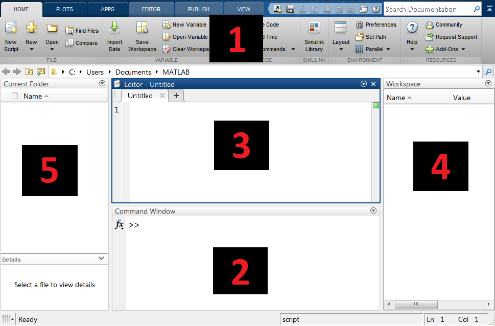
Main window of MATLAB environment is shown below:

All tools are grouped in ribbons, located at the top of the window (1). Command line (2) located at the bottom can be used for interactive calculation by manual command input. More elaborate computation can be done using script files, edited in the central part of the window (3). Workspace with current variables is located on the right (4), and current directory contents are shown on the left (5).
Default layout can always be restored using Layout → Default command, located in Home ribbon:

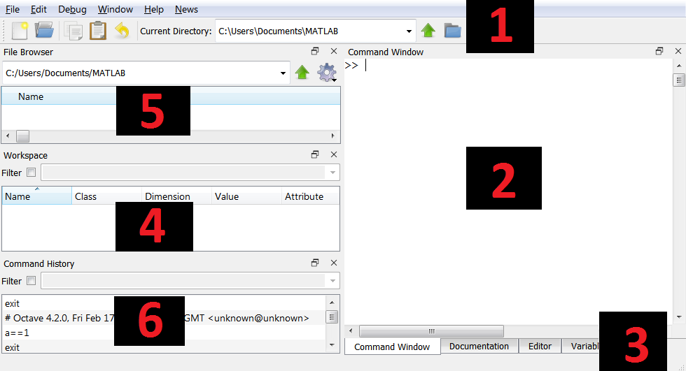
Main window of GNU Octave GUI has a similar layout:

Basic tools are available at the top (1). Command line (2) is located on the right, but can be switched to script editor osing tabs at the bottom (3). On the right, there is a column with three elements, from the top: current directory file browser (5), workspace variables (4) and command history (6).
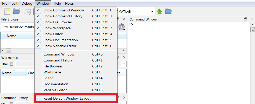
If layout has been changed, it can always be restored using Window → Reset Default Window Layout:

MATLAB basics
Basic mathematical operations
In MATLAB, you can use basic mathematical operators, such as +, -, *, /, keeping order of operations. To force different order, () parentheses can be used:
>> 3 + 5

ans =
     8

>> 9 - 8 * 100

ans =
  -791

>> (9 - 8) * 100

ans =
   100

>> 100 / 6

ans =
   16.6667
Exponentiation can be done using caret operator ^:
>> 2 ^ 16

ans =
       65536
🔨 🔥 Assignment 🔥 🔨
Test all of above operators in MATLAB command line.
A rocket accelerates uniformly with acceleration of 100 m/s^2. Calculate the distance it will travel in 10 seconds. Hint:
All entered commands are saved in history, which can be accessed using up/down arrows on the keyboard. In MATLAB, this causes a history pop-up to appear, in Octave it is always visible on the left. Commands accessed from history can be edited.
🔨 🔥 Assignment 🔥 🔨
Check how history works in MATLAB.
Variables
MATLAB language allows for storing values in variables. Assignment to a variable can be done using = operator. Variable type is chosen automatically based on assigned contents:
>> base = 20

base =
    20

>> height = 3

height =
     3

>> base * height / 2

ans =
    30
Computed results can be saved to a variable:
>> netto = 100

netto =
   100

>> tax = 1.23

tax =
    1.2300

>> brutto = netto * tax

brutto =
   123
String literals are enclosed in single quotes '. If a single quote has to be present in the string itself, it has to be prepended with another one:
>> s1 = 'Anna has a dog'

s1 =
    'Anna has a dog'

>> s2 = 'This is Anna''s dog'

s2 =

    'This is Anna's dog'
🔨 🔥 Assignment 🔥 🔨
- Using command line, assign length of a square diagonal to
dvariable. - Based on
d, calculate length of square side and save in variablea. Hint, remember that calculating square root of a number is the same as raising a number to the power of 0.5.
- Using the result, calculate area of a circle inscribed in the square. Hint π value can be accessed using
picommand.
Vector and matrix operations
Vectors
In MATLAB, a vector can be defined by providing a space-separated list of values enclosed in square brackets []:
>> primes = [2 3 5 7 11 13 17 19 23 29 31 37]To access vector elements, round parentheses () operator can be used. Single elements or ranges can be accessed. Remeber that in contrast to most programming languages, array indexes in MATLAB start at 1:
>> primes(1)

ans =
     2

>> primes(2:5) % right-closed (inclusive) interval

ans =
     3     5     7    11

>> primes(3:end) % interval from 3 to vector end

ans =
     5     7    11    13    17    19    23    29    31    37


>> primes(1:2:end) % every other element

ans =
     2     5    11    17    23    31
Separating values with semicolons ; causes them to be placed in rows, creating a column vector:
>> a = [1; 2; 3; 4]

a =
     1
     2
     3
     4
A signle quote ' can be used to transpose the vector, giving the same effect:
>> a = [1 2 3 4]

a =
     1     2     3     4

>> a'

ans =
     1
     2
     3
     4
Vectors can be concatenated using square brackets []:
>> a = [1 2]

a =
     1     2

>> b = [3 4]

b =
     3     4

>> [a b]

ans =
     1     2     3     4
Vectors can also be created using a : range operator:
>> x = [1:10]

x =
     1     2     3     4     5     6     7     8     9    10
It is also possible to specify step different than 1:
>> t = [0:0.01:1] % creates a vector from 0 to 1 (inclusive)
                  % with 0.01 step (which results in a 101-element vector)

>> z = [10:2:20]  % creates a vector from 10 to 20 (inclusive)
Vectors of compatible sizes can be added and subtracted (+, -):
>> a = [1 2 3 4 5]

a =
     1     2     3     4     5

>> b = [6 7 8 9 10]

b =
     6     7     8     9    10

>> a + b

ans =
     7     9    11    13    15

>> a - b

ans =
    -5    -5    -5    -5    -5
Multiplication on vectors/matrices using * operator is done as a matrix operations. By multiplying a row vector by a column vector, a vector dot product is achieved:
>> a * b'

ans =
   130
Element-wise multiplication can be done using a .* operator:
>> a .* b

ans =
     6    14    24    36    50
Length of a vector can be accessed using length() function:
>> length(a)

ans =
     5
Matrices
In MATLAB matrices are defined similarly to vectors, with each row separated with semicolons (;):
>> y = [1 2 3; 4 5 6; 7 8 9]

y =
     1     2     3
     4     5     6
     7     8     9
Again, elements can be accessed using parentheses operator (), by providing a pair of indexes. The first parameter specifies row(s), the second specifies column(s). Indexing starts at 1:
>> y(1,3)

ans =
     3

>> y(1:2,1:2)

ans =
     1     2
     4     5
Similarly to vectors, basic math operations are supported: +, -, *, .*, /, ./. A matrix can be transposed using a single quote operator '. Remeber that in matrix multiplication, order of arguments matters!
>> y * y'

ans =
    14    32    50
    32    77   122
    50   122   194

>> y' * y

ans =
    66    78    90
    78    93   108
    90   108   126
Vectors and matrices can also be used in math operations with scalars:
>> y * 3

ans =
     3     6     9
    12    15    18
    21    24    27

>> y + 3

ans =
     4     5     6
     7     8     9
    10    11    12
Matrix size can be accesed using size() function. The function returns a two-element vector containing number of rows and columns:
>> c = [1 2 3; 4 5 6]

c =
     1     2     3
     4     5     6

>> size(c)

ans =
     2     3
🔨 🔥 Assignment 🔥 🔨
- Create 3 vertical vectors of length 5, filled with various values. Concatenate them horizontally to create a 5x3 matrix.
- Multiply the resulting matrix by the same matrix, transposed.
- Myltiply the result by 10.
Creating basic matrices
Apart from providing values manually, some matrices can be obtained using dedicated functions. Their arguments are usually matrix dimensions: number of rows and number of columns. Supplying a single argument will result in a single n x n matrix.
>> zeros(3,3) % matrix filled with zeros

ans =
     0     0     0
     0     0     0
     0     0     0

>> ones(2,5) % matrix filled with ones

ans =
     1     1     1     1     1
     1     1     1     1     1

>> eye(4) % identity matrix

ans =
     1     0     0     0
     0     1     0     0
     0     0     1     0
     0     0     0     1

>> rand(2,2) % random values from range <0, 1>

ans =
    0.8147    0.1270
    0.9058    0.9134
🔨 🔥 Assignment 🔥 🔨
Using above functions create a 4 x 6 (rows x columns) matrix filled with value 5.
Math funcitons
MATLAB has a wide range of mathematical functions built-in, below is a very small excerpt of them:
| Function | Description |
|---|---|
| sin(a) | trigonometric functions, arguments in radians |
| cos(a) | |
| tan(a) | |
| cot(a) | |
| sind(a) | trigonometric functions, arguments in degrees |
| cosd(a) | |
| tand(a) | |
| cotd(a) | |
| sqrt(a) | square root |
| exp(a) | natural exponential function (e^a) |
| log(a) | natural logarithm |
| log10(a) | base-10 logarithm |
| abs(a) | absolute value |
Examples:
>> sin(pi/2)

ans =
     1

>> sin([0:5])

ans =
     0    0.8415    0.9093    0.1411   -0.7568   -0.9589
🔨 🔥 Assignment 🔥 🔨
- Create a vector containing integers from -10 to 10.
- Using known functions, create a vector of absolute values of above vector.
- Calculate square root values of above vector.
Executable scrips
During normal MATLAB operation, the commands are rarely input directly in the command line, but rather executed from a text file - a script. Scripts in MATLAB have a .m file extension. A new script can be created using New Script in HOME ribbon. A new script Editor window will be opened. The script can be saved by clicking on Save command in EDITOR ribbon. When choosing a script filename, use only alpahnumeric characters and underscore (_).
🔨 🔥 Assignment 🔥 🔨
- Create a new script.
- Save it as my_first_script.m.
To run a script, click RUN in EDITOR ribbon. Alternatively, press F5 on the keyboard. The script results will be shown in the console.
🔨 🔥 Assignment 🔥 🔨
- Add simple code to the newly created script, for example:
a = 1
b = 4

a * b- Run the script.
By default, MATLAB displays the result of each operation in console. The output can (and usually should) be silenced by adding a semicolon (;) at the end of each command.
🔨 🔥 Assignment 🔥 🔨
- Modify the script so that assignment to variables is not displayed in the console.
- Run the script.
Each script can also be run directly from the command line, by inputting the script name as a command. Similiarly, they can be run from another script.
🔨 🔥 Assignment 🔥 🔨
Run your script from the command line.
Plots
MATLAB provides an easy to use plotting interface. To display a simple 2D plot, a plot(x,y) can be used, by providing two vectors of corresponding XY values. By default the points are connected with straight lines.
🔨 🔥 Assignment 🔥 🔨
- Copy the code below to your script and execute:
x = [1 2 3 4];
y = [1 2 3 4];

plot(x,y,'-o')

grid on- Change
yvalues to[1 2 1 2]. Run the script and see the result. - Change
xvalues to[1 2 2 1]. Run the script. As you can see, the input points don't have to represent a function.
An optional third argument can be provided to change the plot's appearance. It can modify line color and style or specify markers placed in each point. Detailed help of each MATLAB function can be obtained using a doc function command, for example:
doc plot🔨 🔥 Assignment 🔥 🔨
- Using command line, open
plotfunction documentation. - Go to section Input Arguments -> Line Spec.
- Modify the script so that the plot is displayed with a dashed red line, and points are marked with cross symbols.
Subsequent plot calls overwrite current figure contents. This behavior can be changes using below command:
hold onAfter calling hold on, each subsequent plot call will append data to the current figure. The behavior can be reverted using below command:
hold offA new figure window can be created using a figure command:
figureWarning plot and related commands, always use the most recently active figure window.
Other commands useful during plotting:
grid on- adds grid helper line,axis tight- removes extra whitespace around the plot,axis equal- scales the axes proportionally,title('string')- specifies plot title,xlabel('x')- x axis label,ylabel('y')- y axis label,legend('variable1', 'variable2', ...)- adds a legend,xlim([xmin xmax])- sets x axis range,ylim([ymin ymax])- sets y axis range.
Final assignment 🔥 🔨
- In a script, create a time vector
t = [0:0.01:1]. Generate values of sine functions of two frequencies: 2 Hz i 10 Hz, save them in separate variables, and plot. Specify the color lines to green and red, respectively. Add plot title, axis labels, legend, and grid. Set y axis range to -1.2 to 1.2.
Calculate a new vector - sum of previously calculated sinusoidal components. Plot it in the same figure, in blue. Change y axis range to -2.5 to 2.5.
Calculate RMS - root mean square value of the result from previous task. Hint You can use
mean()to calculate mean value of a vector. Note that elements have to be squared.
Homework 💥 🏠
Task 1
A vector x with values [-10:0.01:10] is given. Calculate values of functions described by below polynomials:
Plot both functions in a figure. Find minimal, maximal and mean values of the function, display them in console (Hint: check mean(), min(), max()).
Task 2
Find out how to place more than one chart in a single figure. Start with built-in help:
doc subplotCreate a figure with two plots one below another. Similarly to Tasks 1 and 2 from Final assignment, plot two sine functions (2 Hz i 10 Hz) on the top plot, and their sum on the bottom plot.
Authors: Rafał Kabaciński, Tomasz Mańkowski, Jakub Tomczyński