ROS introduction/recap

Robot Operating System (ROS) is an open-source robotics middleware suite. Although ROS is not an operating system (OS) but a set of software frameworks for robot software development, it provides services designed for a heterogeneous computer cluster such as hardware abstraction, low-level device control, implementation of commonly used functionality, message-passing between processes, and package management.

IMPORTANT: There are two versions of ROS (ROS1 and ROS2) and many distributions. We will be working with ROS1 Noetic. ROS2 has some major differences about which you can read here.

ROS Computation Graph diagram

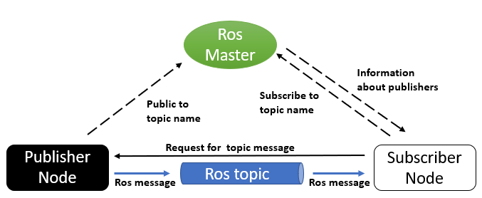
• Nodes: Nodes are processes that perform computation.

• Master: The ROS Master provides name registration and lookup to the rest of the Computation Graph. Without the Master, nodes would not be able to find each other, exchange messages, or invoke services.

• Parameter Server: The Parameter Server allows data to be stored by key in a central location.

• Messages: Nodes communicate with each other by passing messages. A message is simply a data structure, comprising typed fields.

• Topics: Messages are routed via a transport system with publish / subscribe semantics. A node sends out a message by publishing it to a given topic. The topic is a name that is used to identify the content of the message. A node that is interested in a certain kind of data will subscribe to the appropriate topic.

• Services: The publish / subscribe model is a very flexible communication paradigm, but its many-to-many, one-way transport is not appropriate for request / reply interactions, which are often required in a distributed system. Request / reply is done via services, which are defined by a pair of message structures: one for the request and one for the reply.

• Bags: Bags are a format (.bag) for saving and playing back ROS message data.

HINT: You can read more about ROS concepts here.

HINT: Installation instructions for ROS1 can be found here. You can also use official ROS docker images.

Catkin workspace and packages:

While working with ROS, you will be working inside a catkin workspace. Catkin workspace is a folder where you modify, build, and install catkin packages. Workspace lets you build multiple catkin packages together all at once. ROS nodes are written inside the catkin packages.

Before creating a catkin workspace make sure to source the ROS environment setup file to have access to ROS commands:

source /opt/ros/[YOUR_ROS_DISTRO]/setup.bash

To create a catkin workspace you have to create a directory with src folder and run catkin_make:

mkdir -p catkin_ws/src
cd catkin_ws
catkin_make

The catkin packages should reside inside src folder. To build the ROS nodes (catkin packages) you have to run the same command in the same directory as above:

catkin_make

After building you have to source the environment variables. Remember that you have to do that in every terminal in which you want to use the built code. Note that you should do that after every building operation to use newly built code.

source devel/setup.bash

Running nodes:

Before the execution of any node, you have to start a ROS system:

roscore

Running a single node:

rosrun [PACKAGE] [NODE_NAME]

Running a .launch file (with the use of .launch file you can, e.g. run multiple nodes with one command):

roslaunch [PACKAGE] [FILENAME].launch

Working with topics:

Display the list of available topics:

rostopic list

Display the information about a specific topic:

rostopic info [TOPIC]

Read messages published to the topic:

rostopic echo [TOPIC]

Publish message to the topic:

rostopic pub [TOPIC] [MSG_TYPE] [ARGS]

Bags

A bag is a file format in ROS for storing ROS message data. ROS messages can can be recorded inside bag files and played back in ROS. They provide a convenient way for testing the developed code and creating datasets.

Play back the contents of a file:

rosbag play [BAG_FILE_PATH].bag

Display a summary of the contents of the bag file:

rosbag info [BAG_FILE_PATH].bag

HINT: More informations about ROS and more ROS tutorials can be found here.

Point Clouds

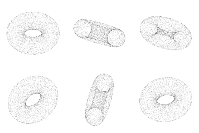
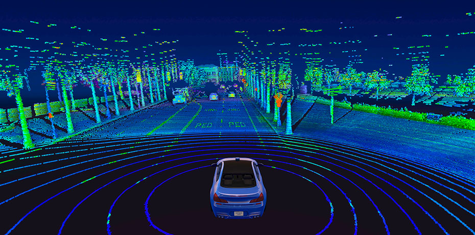
A point cloud is a discrete set of data points in space. The points may represent a 3D shape, object or scene. Each point position has its set of Cartesian coordinates (X, Y, Z). Point clouds are generally produced by 3D scanners, LIDARs or by photogrammetry software.

Example data

Point Cloud Library (PCL)

The Point Cloud Library (PCL) is a standalone, open-source library for 2D/3D image and point cloud processing. The library contains algorithms for filtering, feature estimation, surface reconstruction, 3D registration, model fitting, object recognition, and segmentation. We will use PCL C++ API. There is a small python binding to the PCL library, but is it no longer maintained and the functionalities are limited.

HINT: PCL documentation can be found here.

HINT: PCL tutorials can be found here. Using PCL in ROS is described here.

pcl::PointCloud<PointT> type

pcl::PointCloud<PointT> is the core point cloud class in the PCL library. It can be templated on any of the Point types listed in point_types.hpp, e.g.:

• PointXYZ - float x, y, z coordinates
• PointXYZI - float x, y, z coordinates and intensity
• PointXYZRGB - float x, y, z coordinates and rgb color

The points in the pcl::PointCloud are stored in a points field as a vector.

Clouds in PCL are usually handled using smart pointers, e.g.:

pcl::PointCloud<pcl::PointXYZ>::Ptr pcl_cloud

PCD (Point Cloud Data)

PCD (Point Cloud Data) is the primary data format in PCL. Point cloud can be saved in .pcd format with pcl::io::savePCDFile function. Point clouds saved in .pcd format can be displayed with the use of pcl_viewer command line tool from pcl_tools package. You can test it by downloading the example .pcd file and running the pcl_viewer:

wget https://raw.githubusercontent.com/PointCloudLibrary/pcl/master/test/bunny.pcd
pcl_viewer bunny.pcd

Point cloud in .pcd format can be loaded in code with pcl::io::loadPCDFile function.

The other common data formats for point clouds are: .ply, .las, .obj, .stl, .off.

Usage interface

Most of the PCL's functionalities (e.g., filters, segmentations) follow similar usage interface:

• use .setInputCloud() to set the input cloud
• set functionality-specific parameters with .set...()
• depending on the functionality call .compute(), .align(), .filter(), etc. to get the output.

PassThrough filter example:

(Passthrough filter filters values inside or outside a specified range in one dimension)

pcl::PassThrough<PointT> filter;
filter.setInputCloud(input_cloud);
filter.setFilterFieldName("x");
filter.setFilterLimits(0.0, 5.0);
filter.filter(output_cloud);

Exercises

Data download

Download the .bag files from following links:

• https://drive.google.com/file/d/1BzrYD6691-iUnGSD2Jg6k95rEmkvwUsA/view?usp=sharing
• https://drive.google.com/file/d/1tP4JcVKj01HjQlGjOjdV2N5Dx35lSmZe/view?usp=sharing

Docker container setup

To make things easier the docker image with PCL was prepared.

1. Download the docker image from here

2. Load the image:

docker load < ros_noetic_pcl.tar

2. Add access to desktop environment for docker container

xhost +local:'docker inspect --format='.Config.Hostname' MP_PCL'

3. Run new docker container

docker run -it \
    --net=host \
    --env=DISPLAY=$DISPLAY \
    --env=NVIDIA_VISIBLE_DEVICES=all \
    --env=NVIDIA_DRIVER_CAPABILITIES=all \
    --volume=/tmp/.X11-unix:/tmp/.X11-unix:ro \
    --volume=/home/student/mp_docker:/home/share:rw \
    --env="QT_X11_NO_MITSHM=1" \
    --env="XAUTHORITY=$XAUTH" \
    --volume="$XAUTH:$XAUTH" \
    --privileged \
    --workdir=/home \
    --name=MP_PCL \
    ros_noetic_pcl:latest \
    bash

NOTE: You will be able to exchange the data between the host machine and container using the shared folder: /home/student/mp_docker:/home/share.

4. To attach to a container in different terminal you can run:

docker exec -it MP_PCL bash

ROS package setup

1. Create a catkin workspace.

mkdir -p catkin_ws/src
cd catkin_ws
catkin_make

2. Clone the prepared ROS package to the workspace

cd src
git clone https://github.com/dmn-sjk/mp_pcl.git

3. Build the package and source the environment

cd ..
catkin_make
source devel/setup.bash

Task 1 - Create a range image from point cloud

NOTE: Keep in mind that both PCL and OpenCV had to be installed and configured for the project beforehand.

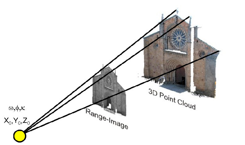
Range images are commonly used representations for 3D LiDAR point cloud processing in the field of autonomous driving. The 2D image view is a more compact representation and can be more convenient to use. The range image is an image on which every pixel is a distance (range) between the obstacle and the sensor.

The task is to fill the pixels of an image with the range values from the LiDAR point cloud to create a range image. The sensor data is from ouster OS1-128 LiDAR. Dimensions of the image (1024x128) refer to parameters of the used LiDAR sensor (horizontal resolution: 1024, vertical resolution: 128). Vertical field of view of the sensor is $\pm$ 22.5 $^\circ$.

How to generate a range image from point cloud?

Tao et al., Detailed Analysis on Generating the Range Image for LiDAR Point Cloud Processing. Electronics 2021, 10, 1224.

Given a point's 3D Cartesian coordindates (x, y, z), we need to calculate the spherical coordinates (the range r, the azimuth angle θ and the elevation angle φ):

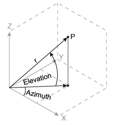
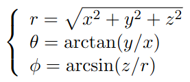
Let u and v represent the column and row index of the range image. Ideally, the center column of the range image should point to the vehicle’s heading direction. Therefore, the column index u can be calculated as:

If we define φ_up and φ_down as the maximum and minimum elevation angles, we have:

Steps:

1. Open src/ex1.cpp file from cloned package (I suggest using the remote explorer extension for VS code to attach to a running container).
2. Calculate the range, horizontal angle (azimuth angle) and vertical angle (elevation angle) of the laser beam for each point. Use atan2 function for arctan calculation to handle angles greater than $\pm$π/2.
3. Calculate the pixel location on the image for each point.
4. If the value of range is higher than 50 m, set it to 50 m.
5. Normalize pixel values from 0-50 to 0-255.
6. To check the results run the roslaunch and play back the LiDAR data recorded in ouster.bag. The range image is published and should be visible in the visuzalization tool rviz.

roslaunch mp_pcl ex1.launch

rosbag play --loop ouster.bag

NOTE: --loop flag makes the rosbag play in a loop.

Expected result:

Task 2 - Detecting the cones in the point cloud with the use of PCL

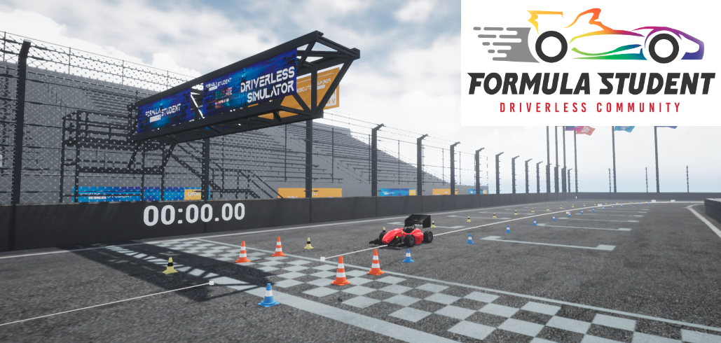
Your task is to detect the cones in the cloud and estimate their center points. The LiDAR data was simulated and recorded from the Formula Student Driverless Simulator.

1. Open src/ex2.cpp file from the cloned package.

2. Complete the filter function to downsample the point cloud (reduce the number of points, to make the point cloud processing faster) with a voxel filter.

   Voxel filter creates a 3D voxel grid (think about a voxel grid as a set of tiny 3D boxes in space) over the input point cloud data. Then, in each voxel (i.e., 3D box), all the points present will be approximated (i.e., downsampled) with their centroid.

   Use pcl::VoxelGrid class. The leaf size (voxel dimensions) can be set with the .setLeafSize() method. Observe how different leaf size values affect the output cloud.

3. Complete the remove_ground function to remove the ground from the point cloud, to be able to segment the cones in the next steps. Since it is the data from simulation with perfectly flat ground, you could just limit the value of points in the Z axis. However, to get familiar with PCL, fit the plane to the point cloud with RANSAC algorithm using pcl::SACSegmentation and extract "inlier points" from the original cloud with pcl::ExtractIndices. The inlier points are the points that approximately lay on the fitted plane (the ground).

4. Complete the get_cluster_indices function. Use Euclidean clustering (pcl::EuclideanClusterExtraction) to cluster points of each cone.

   Euclidean clustering segments a point cloud by grouping points within a specified distance threshold into distinct clusters based on their spatial proximity.

5. Complete get_cones_centers_cloud function. Get a single center point of each cone, by calculating the average position of points in each cone cluster. You can calculate the average of each dimension manually or use pcl::CentroidPoint.

6. To check the results run the roslaunch and playback the data from fsds_lidar.bag:

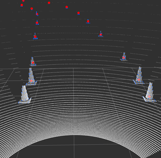
roslaunch mp_pcl ex2.launch

rosbag play --loop fsds_lidar.bag

The final result should look like this (white points - unprocessed cloud, blue points - downsampled cloud without ground points, red points - centers of cones):